-
Site
- Administrator Guide
- Usage Quickstart
- Metric Shell
- Developers Manual
- Highchart demo in sphinx
- TODO
- Directory Structure
- File contents
- UBMoD
- Stand Allone Web Server
- Page
- « Administrator Gu...
- Developers Manua... »
Cloud Metrics supports a convenient shell to aide in the cloud usage data analysis. It is advisable that users use the shell in case you like to conduct multiple analysis steps. The shell is designed to read a user’s input, calculate metrics data, and then provide the results in an appropriate format such as a standard output, JSON, JPG, PNG, and html with javascript charting libraries embedded
To activate the metric shell please execute the command:
$ fg-metric
Once you do this you can issue some of the metric shell commands. Here is a simple example that analyzes the runtime metric for a machine india on which openstack is installed and prints a chart:
set nodename india
set platform openstack
set metric runtime
analyze
chart
Before performing an analysis, several settings need to be specified with the set command. This command allows to associate one or more values with a key:
fg-metric> set $key $value[ $value2 ...]
To analyze data between these two dates please set the date range:
fg-metric> set date 2012-01-01T00:00:00 2012-12-31T23:59:59
To specify which metric item will be calculated please set it as follows:
fg-metric> set metric runtime

(multiple metrics)
fg-metric> set metric runtime count
We are supporting the following metrics:
fg-metric> set metric help
Possible commands
=================
 set metric count
 set metric runtime
 set metric countusers
 set metric cores
 set metric runtimeusers
 set metric memories
 set metric disks
As our metric system can handle multiple coulds, it is important to set for which host the calculations are to be specified. Please set it ass follows where the name india is your machine that holds the IaaS:
fg-metric> set hostname india
To specify which cloud service will be included please use the following command:
fg-metric> set platform openstack
The help command is useful to obtain a simple help message for the available commoand:
fg-metric> help

Documented commands (type help <topic>):
========================================
_load           clear           edit     l     pause    run      shell
_relative_load  cmdenvironment  get      li    py       save     shortcuts
analyze         csv             hi       list  r        set      show
chart           ed              history  load  refresh  setconf  showconf

Undocumented commands:
======================
EOF  eof  exit  help  q  quit
Todo
document the undocumented commands and include new output here once done.
To find out more details about an available shell command, simply type in help followed by the command:
fg-metric> help set
Set a function with parameter(s)

fg-metric> set help

Possible commands
=================
set date $from $to
set metric $name
set platform $name
set nodename $name
To ask for help for a parameter you can do this as follows (here we give an example for finding mor out about the set data command:
fg-metric> set date help
Usage: set date from_date(YYYY-MM-DDTHH:MM:SS) to_date(YYYY-MM-DDTHH:MM:SS).
(e.g. set date 2012-01-01T00:00:00 2012-12-31T23:59:59)
Todo
Hyungro
Once you conducted an analyze, cloud metrics supports several output options such as stdout, JSON, csv, jpg, png, html that can be created with the help of various commands such as chart and csv which we describe next.
Todo
Hyungro, what about the other commands? I do not think they are listed here.
chart is a command to create a chart html file with different chart types (e.g. bar, line, column, etc.). To help understanding of data, a type of charts should be selected carefully. Relationships between data and chart type refer to proper representation.
Assume, the data is:
Example usage of the chart command:
fg-metric> ...(skipped)...
fg-metric> analyze
fg-metric> chart -t pie-basic --directory $directory_name
csv ia a command to export statistics as a comma-separated values (csv) file.
Example usage of csv command:
fg-metric> ...(skipped)...
fg-metric> analyze
fg-metric> csv
2012-01-01T00:00:00-2013-01-01T00:00:00-runtime-openstack-india-dailyAll.csv is created

(or)
fg-metric> csv -o test/result.csv
test/result.csv is created
We show now some examples to highlight how easy it is to generate statistics with the metric shell.
This example shows you how to retrieve data for a certain time period. set period daily provides statistics grouped by date. For example, if the date settings cover 30 days, the statistics will have 30 record sets instead of a single record. The chart type can be selected with chart -t option. line-time-series is one of the types in highcharts. For more details of the types, see here: Highchart Demo. In our example we create a chart that represents for each day the number of users using a cloud services in a histogram over the specified period (see Figure 1). Using the script:
clear
set nodename sierra
set date 2012-10-01T00:00:00 2012-12-31T23:59:59
set period daily
set metric countusers
analyze
chart -t line-time-series --directory 2012-Q4/
will result in the following image:
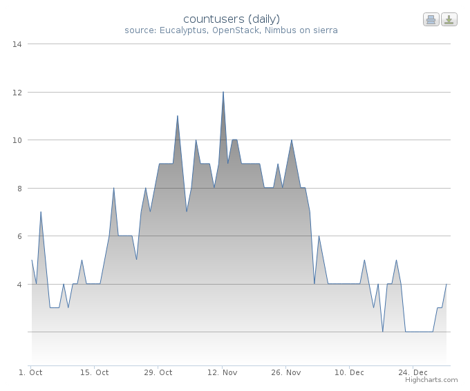
Figure 1. The count of active users.
This example represents data in percentages for different project groups. In this example, we use groupby instead of period in the previous example. It will result in a pie chart showing the fractions of Launched VM instances by Project groups (Figure 2). Using the script:
clear
set nodename sierra
set date 2012-10-01T00:00:00 2012-12-31T23:59:59
set groupby project
set metric count
analyze
chart -t pie-basic --directory 2012-Q4/
will result in the following image:
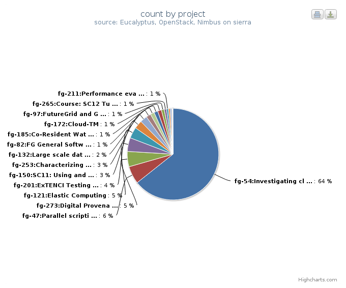
Figure 2. VMs count by Project.
This example represents multiple data in a single chart with multiple axes. combo-multi-axes allows to depict three metrics in a single chart. Here we show a chart that includes average monthly usage as to Wall Hour (runtime), Count and the number of Users for VM instances (Figure 3). Using the script:
clear
set nodename sierra
set date 2012-10-01T00:00:00 2012-12-31T23:59:59
set period monthly
set metric runtime count countusers
set timetype hour
analyze
chart -t combo-multi-axes --directory 2012-Q4/
will result in the following image:
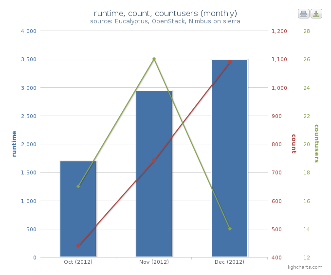
Figure 3. Average Monthly Usage Data (Wall hour, Launched VMs, Users)
The following will create a table with data produced for the month of January:
> fg-metric
fg> clear users
fg> analyze -M 01
fg> table --type users --separator ,  --caption Testing_the_csv_table
fg> quit
Naturally you could store this script in a file and pipe to fg-metric in case you have more complex or repetitive analysis to do.
Note
TOODO: Why is this eucalyptus?
Note
TOODO: Why not ” ” in -t argument?
Assume you like to create a nice html page directory with the analysis of the data contained. This can be done as follows. Assume the following contents is in the file analyze.txt:
clear users
analyze -M 01 -Y 2012
createreport -d 2012-01 -t Running_instances_per_user_of_Eucalyptus_in_India

clear users
analyze -M 02 -Y 2012
createreport -d 2012-01 -t Running_instances_per_user_of_Eucalyptus_in_India

createreports 2012-01 2012-02
This page creates a beautiful report page with links to the generated graphs contained in the directories specified. All index files in the directories are printed before the images in the directory are included. The resulting report is an html report.
To start the script, simply use:
cat analyze.txt | fg-metric
This will produce a nice directory tree with all the data needed for a display.
Note
TOODO: Hyungro do the test and complete, this will help you getting your automatic example going
Note
TOODO: Why is this eucalyptus?
The previous example has the disadvantage that one has to explicitly copy the lines that we use to access the analysis. However as Python includes loops, we can just use loops to create such a script programatically, while changing some parameters at the beginning:
#! /usr/bin/env python
from sh import fg-metric as metric

filename = "/tmp/analyze.txt"

years = ['2013']
months =['01', '02']

script = """
clear users
analyze -M %s(month) -Y %s(year)
createreport -d %s(year)-result -t Running_instances_per_user_of_Eucalyptus_in_%s(host)
"""
###############################
# DO NOT CHANGE FRM HERE
#
# Assampble the anzlyses to be done

f = open (filename, "w")

for year in years:
  for  month in months:
     data = {"year": year, "month": month}
     print >>f, script % data
close f
# finish the script

metric("-f", filename)
Naturaly this programm pattern can be used for more cases such as identifying the current time and generating based on this scripts the automatically create new alanysis, or the detection if an analysis was already performed and skipping it. Hence it is possible to create a fast script that does not need to recreate the majority of the calculations, but only injects new data and calculate metrics based on this new data.